multiplex wormhole

The Optimization Process

In silico optimization of multiplex PCR primers is the foundation of multiplex wormhole. The basic optimization algorithm relies on an iterative process where an initial set is designed, then at each iteration, a primer pair is randomly swapped with an alternative. If the dimer load of the multiplex improves based on this swap, the change is kept for the next iteration, otherwise the change is discarded. The process is repeated until either 1) a dimer load of 0 is achieved, 2) all alternative changes are tested and shown to provide no further improvement, or 3) the maximum number of iterations (set by the user) is reached.

Cost Functions

multiplex_wormhole can describe “dimer load” using two distinct cost functions:

With the standard approach (deltaG=False), cost of the multiplex is calculated as the total count of dimers between primer pairs within the set. The cost table for this approach can be either the count of dimers per pairwise interaction (i.e., to minimize for total dimer load) or a binary pairwise table indicating which primer pairs interact (i.e., to minimize the number of interacting pairs). By default with this approach, multiplex wormhole minimizes total dimer load.

Alternatively, with the deltaG approach (deltaG=True), cost of the multiplex reflects the “badness” or strength of dimers within the multiplex. For each combination of primer pairs, the minimum deltaG (i.e., worst or strongest) is identified. Then, this is averaged across pairwise combinations within the multiplex. The maximum “mean deltaG” (i.e., closest to zero - reflecting weakest dimers) is then optimized for.

For simple problems, both approaches will return a final predicted dimer load of zero. However, for complex problems where dimerization is inevitable, the deltaG option allows strength of dimers to be considered rather than treating all dimers equally. This may be particularly valuable when building large multiplexes.

Optimization Procedure

1. Selecting an initial primer set: Greedy algorithm

An initial set of primer pairs is selected by using a pseudo-greedy algorithm that considers one template at a time:

1. The “best” primer pairs are identified for each template based on having the lowest cumulative dimer load (sum of dimers or mean deltaG) across all candidate primer pairs.
2. Next, the best per-template primer pairs are sorted from lowest to highest cumulative dimer load.
3. Then, an initial set of N_LOCI primer pairs is selected by choosing the “best” from the above sorted list of “best” per-template primer pairs. If a keeplist is provided, the keeplist primer pairs are included in the initial set and N_LOCI-N_KEEPLIST_PAIRS “bests” are chosen.

2. Minimizing dimer load: Simple iterative improvement algorithm

The initial set is then used as input for a simple iterative improvement algorithm. At each iteration, the total and per-pair costs (i.e., dimer load) are calculated for the current multiplex. Then, the following steps are taken:

1. The “worst” primer pair within the current set is identified and swapped with a random alternative. The total cost is calculated for this new set.
2. If the new total cost is lower than the previous total cost, then the change is kept and the algorithm proceeds to the next iteration.
3. If cost is not reduced, then the algorithm will test other alternatives to replace the current worst pair until either 1) an improvement is made or 2) alternatives are exhausted. If alternatives are exhausted, the algorithm will proceed to try to replace the “next worst” primer pair at the next step, and so on.
4. When an alternative is found, the algorithm will proceed to the next iteration. Each iteration starts by trying to replace the “worst” primer pair.
5. This process continues until either A) the primer set is fully optimized (0 dimers), B) no alternatives can improve the set further, or C) the user-defined number of iterations SIMPLE have been run.

This step is where the bulk of reduction in dimer load will occur.

3.Overcoming local minima: Adaptive simulated annealing algorithm

Simulated annealing is an optimization procedure that allows the algorithm to make “mistakes” as it proceeds. Short-term “mistakes” (i.e., changes that result in higher cost) enable the algorithm to overcome local minima in the optimization space using “hill-climbing” behavior. Simulated annealing proceeds along a schedule where riskier decisions (i.e., those resulting in increased cost) are allowed with higher probability in early iterations in order to explore the search space, and with decreasing probability as the algorithm proceeds. Simulated annealing takes the following steps:

The Process

1. Similar to simple iterative improvement, primer pairs are swapped at each iteration. However, in the simulated annealing algorithm, the primer pairs that are swapped are selected randomly.
2. The total dimer load (i.e., cost) of the new primer set is calculated and compared to the cost of the previous set. All changes that improve the primer set (i.e., lower dimer cost) are accepted, while changes that increase cost will be accepted based on a probability function that is defined by the simulated annealing temperature schedule and the change in cost: p = e^(-_PROB_ADJ_ * delta_cost / T) where T is the simulated annealing temperature at the current iteration, delta_cost is the new cost minus the previous cost, and PROB_ADJ is a scaling parameter set by the user (Default=2).
3. The simulated annealing temperature is reduced before proceeding to the next iteration, so that increased costs are less likely to be accepted as the algorithm progresses. The temperature schedule within multiplex wormhole is defined by a geometric function: (T_INIT-T_FINAL)*_DECAY_RATE_**(i_scaled)+T_FINAL where T_INIT is the initial temperature, T_FINAL is the final temperature, i_scaled is the percent of iterations run (i.e., i / (ITERATIONS/100)), and _DECAY_RATE_ is the user-defined temperature decay rate (Default=0.95). See below for details on calculating T_INIT & T_FINAL for each cycle.
4. Steps 1-3 are repeated until ITERATIONS is reached.
5. The simulated annealing cycle ends when the number of iterations is reached. Then, the temperature schedule is restarted and recalculated (details below) and a new simulated annealing cycle is run until the number of CYCLES is reached (Default=10).

The default temperature schedule and acceptance probabilities are plotted on the Exploring Optimization Parameters page.

Defining the Temperature Schedule

In multiplex_wormhole, an adaptive simulated annealing approach is used to set the temperature schedule, where the initial temperature is set based on the cost space of the problem at hand. The initial temperature is recalculated for each simulated annealing cycle (i.e., to account for the change in cost space from the previous cycle) using the following steps:

1. Random swaps (without accepting changes) are sampled for BURNIN iterations (default=200), and the change in cost delta_cost recorded.
2. The MEAN_DIMERS (i.e., mean delta_costs) and MAX_DIMERS (i.e., max delta_costs) are recorded.

3. The initial temperature is calculated based on the ratio of these two values: For deltaG=False : T_INIT = -2*log10( MEAN_DIMER / MAX_DIMER ) + 2, T_INIT<0.3 --> T_INIT=0.3

   For deltaG=True : T_INIT = [-2*log10(MEAN_DIMER / MAX_DIMER) + 1] / 10, T_INIT<0.03 --> T_INIT=0.03 Values are given these lower limits to allow some hill-climbing.

4. The final temperature is set as provided. By default, this value is nearly 0 so that the end of each cycle is running simple iterative improvement: T_FINAL = 0.001

Here’s a plot showing the functional form of T_INIT based on common MEAN_DIMER & MAX_DIMER values:

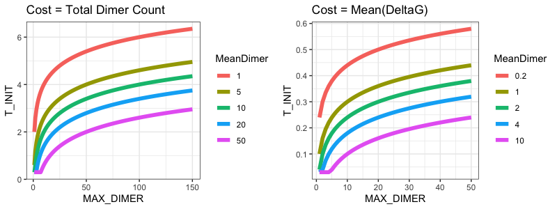
This plot shows the following key characteristics:

• T_INIT increases as MAX_DIMER increases on a logarithmic scale, allowing for higher temperatures with higher observed maximum costs (i.e., higher probability of accepting large changes) but with this effect based on the order of magnitude of MAX_DIMER.
• The T_INIT function shifts upwards with lower MEAN_DIMER, allowing higher acceptance of “mistakes” with mean cost space. This allows the algorithm to accept more “risk” as the cost space includes lower-cost changes and a higher proportion of changes that will reduce cost.
• The minimum value is near 0-2, while the maximum value is <8. Based on testing, values >10 resulted in increased dimer loads as the algorithm progressed.
• Temperatures are lower for the deltaG algorithm. The costs are calculated differently, and deltaG optimization has a more convex solution space which makes runaway hill-climbing more likely.

Users may also choose to set a fixed temperature schedule using the T_INIT and T_FINAL arguments; these will be carried into all simulated annealing cycles. T_INIT between 2-3 (or 0.2-0.3 for deltaG=True) seems to work well for most problems.

Understanding the Dimer Trace Plot

Each multiplex wormhole run will output a dimer trace plot, with the number of iterations based on the total iterations passed (SIMPLE + ITERATIONS), which allows visualization of the contributions of each algorithm. This can also be plotted in R using the _costTrace.csv output. The trace plot can help troubleshoot simulated annealing parameterization:

• Were local optima overcome? Are there small “hills” in the plot at the iterations corresponding to the start of each simulated annealing cycle? If so, hill-climbing is working. Otherwise, if there are no hills or the hills are small, try increasing T_INIT to allow higher hills to be climbed at the start of each cycle. To extend the hill-climbing period of each cycle, increase the DECAY_RATE (e.g., 0.98).
• Was hill-climbing excessive? If the trace plot shows runaways cost increases as simulated annealing progresses, too many cost increases are being accepted. This can be rectified by reducing T_INIT or PROB_ADJ to reduce the probability of accepting large cost increases, or reducing the DECAY_RATE (e.g., 0.90) to make the hill-climbing period of each cycle shorter.
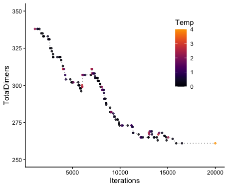
• Is further optimization warranted? There should be less change in cost as the algorithm proceeds (i.e., the plot should start looking more and more like a flat line. If this is not the case, then more optimization is possible. You can run the output back through the optimization step using the SEED argument in both the multipleOptimizations and optimizeMultiplex functions.
• How did temperatures contribute to behavior? If you load _costsTrace.csv into R and plot with (x=Iterations, y=TotalDimers, color=ASA_Temp), you can check which temperatures contributed to changes (good or bad). Example below (truncated to highlight simulated annealing portion):

Additional Tips & Tricks

• See the plot_SA_temps script to test the effects of DECAY_RATE, T_INIT, T_FINAL, and PROB_ADJ on the probability of accepting a range of dimer values as the simulated annealing algorithm proceeds.
• The optimization process is inherently random and results will vary across runs. As such, it’s recommended to run multiple times and select the “best” result. multiple_run_optimization provides an easy wrapper for running and summarizing across multiple runs with standard inputs. Variability in results will increase with problem complexity, and more runs are recommended for very complex problems.
• For simple problems (e.g., selecting 50 primer pairs from 200 candidates), the iterative improvement is sufficient and more efficient. To run the simple iterative improvement algorithm, set SIMPLE high and ITERATIONS=0 to bypass simulated annealing.
• For challenging problems (e.g., many options and/or many N_LOCI), you may consider successive optimization runs. The SEED argument in the optimizeMultiplex function is provided to allow an output from a previous run to be used as the “initial panel” for a new optimization run. This is not the same as just increasing the number of iterations because the simulated annealing temperature schedule will be recalculated for this set and simulated annealing will possibly allow local minima to be overcome.
• When panels are designed to provide multiple levels of information (e.g., individual ID + sex + hybrid status), multiple optimization runs will be necessary to get the desired information content for each inferential objective.
• Optimization is constrained by the number of options available relative to the number of primer pairs desired. The number of candidates required to design a panel with minimal dimer load drastically increases as desired panel size increases.
• One way to test if any hills remain to climb is to rerun optimizeMultiplex with the output as SEED and a high T_INIT (e.g., T_INIT=10). If no improvements are made at this higher T_INIT, you can be sure that you have reached a solution near the global minima (which is unlikely to be truly reached in complex problems).

This site is open source. Improve this page.